"데이터"가 아니라 "문제"를 먼저 보는 연습
이번 분석은 임의의 문제 상황을 가정하고 데이터를 통해 문제를 해결할 방법을 찾는다. 처음에는 의식적으로 '데이터'에 집중하게 되는데 본문에서 일부러 상황과 문제를 계속해서 강조했다. 그러니 '문제'에 집중해보자. '문제'를 이해하면 데이터는 자연스럽게 눈에 들어온다. 특히 후반부에 집단 군집 분석을 진행할 텐데, 이를 위해 머신러닝도 사용해볼 예정이다.
목차
___
Step 1. 문제 상황 가정 및 데이터 전처리
     1-1. 라이브러리 호출 및 데이터 확인
     1-2. 일부 컬럼 제거
     1-3. 컬럼명, 데이터타입 형식 통일
     1-4. 현재 날짜 가정
     1-5. 이상치 처리
1. 문제 상황 가정 및 데이터 전처리
지금부터 우리는 이커머스 스타트업의 데이터 분석가다. 상품이 많아지면서 사용자 수가 늘고 매출 규모는 늘어나고 있지만 최근에 고객들이 많이 이탈하고 있다. 이탈을 막기 위해 방안을 모색하던 중 상품 MD와 플랫폼 기획 쪽에서 서비스 개편이나 상품 수급 기준을 높이자는 의견이 나왔다. 하지만 우리가 볼 때 신규 유입자 수는 역대 최고치를 경신하고 있기 때문에 서비스를 전면 개편하거나 유통업체를 바꾸는 시도는 하지 않는 것이 좋은 상황인 것 같다.
대신 우리는 사용자 수가 기존 대비 가파르게 늘고 있지만 그간 광고 프로모션에는 큰 변화를 주지 않았기 때문에 본인의 소비 성향과 관련 없는 광고에 피로감을 느꼈다고 생각했다. 그래서 기존 고객들이 이탈하고 있는 이유를 서비스가 마음에 들지 않아서가 아니라 광고에 대한 피로감 때문이라는 가설을 세우고 프로모션 A/B 테스트를 통해 검증해보자는 의견을 냈다.
다행히 현업에서도 우리 의견에 공감하여 A/B 테스트 설계를 시작한 상황이다. 실험은 기존의 일괄적인 프로모션과 개인화된 프로모션으로 제작하고, 소비자 그룹을 무작위로 50:50으로 나눠 한쪽은 일괄 프로모션(A), 다른 한쪽은 개인화 프로모션(B)을 적용할 것이다. 이번 분석(광고 프로모션 효율 증진을 위한 커머스 고객 세분화)의 흐름은 개인화 프로모션(B)을 제작하기 전, 개인화(grouping) 기준을 설정해나가는 과정이 되겠다.
1-1. 라이브러리 호출 및 데이터 확인
여건상 캐글 사이트에서 데이터셋을 빌려오자. 대신, 실무 상황을 가정하기 위해 데이터셋을 약간 조정할 것이고 조금은 부족한 데이터셋으로 고객 그룹을 나눠볼 예정이다. 단, 데이터 양이 많지 않기 때문에(2240 rows) 결측치를 일부러 만들거나 하지는 않겠다. 데이터셋은 아래 링크에서 확보했다.
# 데이터프레임
import pandas as pd

# 시간 계산
import datetime

# 시각화
import matplotlib.pyplot as plt
import seaborn as sns
import missingno as msno
# 'Tab' 구분자로 나뉜 csv 파일을 불러온다.
customer_df_r = pd.read_csv('./data/marketing_campaign.csv', delimiter='\t')
customer_df_r.head()| ID | Year_Birth | Education | Marital_Status | Income | Kidhome | Teenhome | Dt_Customer | Recency | MntWines | ... | NumWebVisitsMonth | AcceptedCmp3 | AcceptedCmp4 | AcceptedCmp5 | AcceptedCmp1 | AcceptedCmp2 | Complain | Z_CostContact | Z_Revenue | Response | |
|---|---|---|---|---|---|---|---|---|---|---|---|---|---|---|---|---|---|---|---|---|---|
| 0 | 5524 | 1957 | Graduation | Single | 58138.0 | 0 | 0 | 04-09-2012 | 58 | 635 | ... | 7 | 0 | 0 | 0 | 0 | 0 | 0 | 3 | 11 | 1 |
| 1 | 2174 | 1954 | Graduation | Single | 46344.0 | 1 | 1 | 08-03-2014 | 38 | 11 | ... | 5 | 0 | 0 | 0 | 0 | 0 | 0 | 3 | 11 | 0 |
| 2 | 4141 | 1965 | Graduation | Together | 71613.0 | 0 | 0 | 21-08-2013 | 26 | 426 | ... | 4 | 0 | 0 | 0 | 0 | 0 | 0 | 3 | 11 | 0 |
| 3 | 6182 | 1984 | Graduation | Together | 26646.0 | 1 | 0 | 10-02-2014 | 26 | 11 | ... | 6 | 0 | 0 | 0 | 0 | 0 | 0 | 3 | 11 | 0 |
| 4 | 5324 | 1981 | PhD | Married | 58293.0 | 1 | 0 | 19-01-2014 | 94 | 173 | ... | 5 | 0 | 0 | 0 | 0 | 0 | 0 | 3 | 11 | 0 |
5 rows × 29 columns
결측치와 데이터 타입을 살펴보자.
customer_df_r.info()<class 'pandas.core.frame.DataFrame'>
RangeIndex: 2240 entries, 0 to 2239
Data columns (total 29 columns):
# Column Non-Null Count Dtype
--- ------ -------------- -----
0 ID 2240 non-null int64
1 Year_Birth 2240 non-null int64
2 Education 2240 non-null object
3 Marital_Status 2240 non-null object
4 Income 2216 non-null float64
5 Kidhome 2240 non-null int64
6 Teenhome 2240 non-null int64
7 Dt_Customer 2240 non-null object
8 Recency 2240 non-null int64
9 MntWines 2240 non-null int64
10 MntFruits 2240 non-null int64
11 MntMeatProducts 2240 non-null int64
12 MntFishProducts 2240 non-null int64
13 MntSweetProducts 2240 non-null int64
14 MntGoldProds 2240 non-null int64
15 NumDealsPurchases 2240 non-null int64
16 NumWebPurchases 2240 non-null int64
17 NumCatalogPurchases 2240 non-null int64
18 NumStorePurchases 2240 non-null int64
19 NumWebVisitsMonth 2240 non-null int64
20 AcceptedCmp3 2240 non-null int64
21 AcceptedCmp4 2240 non-null int64
22 AcceptedCmp5 2240 non-null int64
23 AcceptedCmp1 2240 non-null int64
24 AcceptedCmp2 2240 non-null int64
25 Complain 2240 non-null int64
26 Z_CostContact 2240 non-null int64
27 Z_Revenue 2240 non-null int64
28 Response 2240 non-null int64
dtypes: float64(1), int64(25), object(3)
memory usage: 507.6+ KB칼럼이 많아서 한 번에 다 보여주지 못한다. 가로로 늘어뜨린 barplot으로 결측치를 확인해보자.
msno.bar(customer_df_r);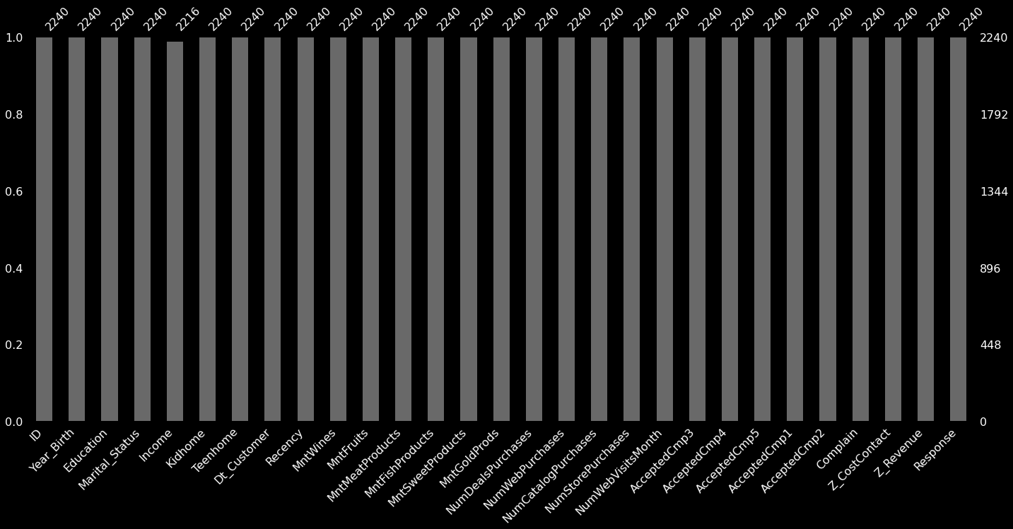
Income 칼럼에만 결측가 보인다. 과연 그런지 조건식을 통해 체크해보자.
# 전체 결측치와 Income 컬럼의 결측치 수를 비교. 일치하면 True 반환
customer_df_r.isnull().sum().sum() == customer_df_r['Income'].isnull().sum()True전체 중 Income 칼럼에만 결측치가 존재한다. 그래서 저 결측치만 적절히 처리해주고 분류 모델에 욱여넣으면 될 것 같은데, 좀 더 현실적인 상황을 만들어보고 싶다.
1-2. 일부 칼럼 제거
머신러닝은 이렇게 양질의 데이터와 독립적인 칼럼들이 많을수록 성능이 좋다. 하지만 실무에서 이렇게 조건이 좋기는 어렵다.
----------------------------------------------------------------------------------
People
----------------------------------------------------------------------------------
ID: Customer's unique identifier
Year_Birth: Customer's birth year
Education: Customer's education level
Marital_Status: Customer's marital status
Income: Customer's yearly household income
Kidhome: Number of children in customer's household
Teenhome: Number of teenagers in customer's household
Dt_Customer: Date of customer's enrollment with the company
Recency: Number of days since customer's last purchase
Complain: 1 if customer complained in the last 2 years, 0 otherwise
----------------------------------------------------------------------------------
Products
----------------------------------------------------------------------------------
MntWines: Amount spent on wine in last 2 years
MntFruits: Amount spent on fruits in last 2 years
MntMeatProducts: Amount spent on meat in last 2 years
MntFishProducts: Amount spent on fish in last 2 years
MntSweetProducts: Amount spent on sweets in last 2 years
MntGoldProds: Amount spent on gold in last 2 years
----------------------------------------------------------------------------------
Promotion
----------------------------------------------------------------------------------
NumDealsPurchases: Number of purchases made with a discount
AcceptedCmp1: 1 if customer accepted the offer in the 1st campaign, 0 otherwise
AcceptedCmp2: 1 if customer accepted the offer in the 2nd campaign, 0 otherwise
AcceptedCmp3: 1 if customer accepted the offer in the 3rd campaign, 0 otherwise
AcceptedCmp4: 1 if customer accepted the offer in the 4th campaign, 0 otherwise
AcceptedCmp5: 1 if customer accepted the offer in the 5th campaign, 0 otherwise
Response: 1 if customer accepted the offer in the last campaign, 0 otherwise
----------------------------------------------------------------------------------
Place
----------------------------------------------------------------------------------
NumWebPurchases: Number of purchases made through the company’s web site
NumCatalogPurchases: Number of purchases made using a catalogue
NumStorePurchases: Number of purchases made directly in stores
NumWebVisitsMonth: Number of visits to company’s web site in the last month
여기서 어느 회사에나 있는 데이터는 다음과 같다.
- People 유형의 고객 ID, 출생연도(Year_Birth), 가입일(Dt_Customer), 가장 최근 구매일(Recency, 여기서는 구매 후 오늘까지 날짜로 저장되어 있다.), 클레임 수(Complain) 칼럼
- Promotion 유형의 모든 칼럼(할인받고 구매한 상품 수와 프로모션에 대한 동의 여부)
- Place 유형의 모든 칼럼(다양한 홍보 채널의 구매 상품 수 관련)
이렇게 상품에 대한 정보, 구매 경로, 고객 가입 정보 등은 어느 업체나 매출 관리를 위해 보유하고 있다.
반면 아래 칼럼들은 설문과 같은 임의의 특정 방식으로 수집하지 않는다면 보유하기 어렵다.
- People 유형의 교육 수준(Education), 결혼 여부(Marital_Status), 소득 수준(Income), 10세 미만 자녀 수(Kidhome), 10대 자녀 수(Teenhome)
- Products 유형의 모든 칼럼(고객이 1년에 어떤 제품을 얼마나 소비하는지 여부, 이 데이터는 소비는 자사 제품의 구매 내역이 아닌 개인 소비 성향에 대한 답변으로 확보된 것으로 보인다.)
우리는 일반적인 회사에 기본적으로 수집하고 있을 법한 데이터만 분석에 사용하겠다. 따라서 사용하지 않을 칼럼들을 모두 제거한다. 추가로, Z_CostContact와 Z_Revenue칼럼은 그 의미가 불분명해 역시 제거한다.
# 혹시 중요한 컬럼이 있을지 모르니 원본은 남겨두고 다른 변수에 새롭게 할당하여 사용한다.
customer_df = customer_df_r.drop(columns=['Education','Marital_Status','Income','Kidhome','Teenhome',\
                                          'MntWines','MntFruits','MntMeatProducts','MntFishProducts','MntSweetProducts','MntGoldProds',\
                                          'Z_CostContact','Z_Revenue'], axis=1)
customer_df.head()| ID | Year_Birth | Dt_Customer | Recency | NumDealsPurchases | NumWebPurchases | NumCatalogPurchases | NumStorePurchases | NumWebVisitsMonth | AcceptedCmp3 | AcceptedCmp4 | AcceptedCmp5 | AcceptedCmp1 | AcceptedCmp2 | Complain | Response | |
|---|---|---|---|---|---|---|---|---|---|---|---|---|---|---|---|---|
| 0 | 5524 | 1957 | 04-09-2012 | 58 | 3 | 8 | 10 | 4 | 7 | 0 | 0 | 0 | 0 | 0 | 0 | 1 |
| 1 | 2174 | 1954 | 08-03-2014 | 38 | 2 | 1 | 1 | 2 | 5 | 0 | 0 | 0 | 0 | 0 | 0 | 0 |
| 2 | 4141 | 1965 | 21-08-2013 | 26 | 1 | 8 | 2 | 10 | 4 | 0 | 0 | 0 | 0 | 0 | 0 | 0 |
| 3 | 6182 | 1984 | 10-02-2014 | 26 | 2 | 2 | 0 | 4 | 6 | 0 | 0 | 0 | 0 | 0 | 0 | 0 |
| 4 | 5324 | 1981 | 19-01-2014 | 94 | 5 | 5 | 3 | 6 | 5 | 0 | 0 | 0 | 0 | 0 | 0 | 0 |
1-3. 칼럼명, 데이터 타입 형식 통일
이어서 칼럼명이 복잡하니 이해하기 쉽도록 네이밍을 조금 수정하겠다.
- 오탈자 방지를 위해 소문자만 사용한다.
- f는 from의 약자, promo는 promotion의 약자로 사용한다.
customer_df.columns = ['id', 'birth', 'enroll', 'day_f_buy', \
                       'buy_f_promo', 'buy_f_web', 'buy_f_catalog', 'buy_f_store',\
                       'visit_web','promo3','promo4','promo5','promo1','promo2','complain','promo6']
customer_df.head()| id | birth | enroll | day_f_buy | buy_f_promo | buy_f_web | buy_f_catalog | buy_f_store | visit_web | promo3 | promo4 | promo5 | promo1 | promo2 | complain | promo6 | |
|---|---|---|---|---|---|---|---|---|---|---|---|---|---|---|---|---|
| 0 | 5524 | 1957 | 04-09-2012 | 58 | 3 | 8 | 10 | 4 | 7 | 0 | 0 | 0 | 0 | 0 | 0 | 1 |
| 1 | 2174 | 1954 | 08-03-2014 | 38 | 2 | 1 | 1 | 2 | 5 | 0 | 0 | 0 | 0 | 0 | 0 | 0 |
| 2 | 4141 | 1965 | 21-08-2013 | 26 | 1 | 8 | 2 | 10 | 4 | 0 | 0 | 0 | 0 | 0 | 0 | 0 |
| 3 | 6182 | 1984 | 10-02-2014 | 26 | 2 | 2 | 0 | 4 | 6 | 0 | 0 | 0 | 0 | 0 | 0 | 0 |
| 4 | 5324 | 1981 | 19-01-2014 | 94 | 5 | 5 | 3 | 6 | 5 | 0 | 0 | 0 | 0 | 0 | 0 | 0 |
# 컬럼별 데이터타입 확인
customer_df.dtypes
id int64
birth int64
enroll object
day_f_buy int64
buy_f_promo int64
buy_f_web int64
buy_f_catalog int64
buy_f_store int64
visit_web int64
promo3 int64
promo4 int64
promo5 int64
promo1 int64
promo2 int64
complain int64
promo6 int64
dtype: objectenroll 칼럼은 내용에 맞게 datetime으로 변경해주자. 그 후 오늘 날짜(가정)와 비교해서 가입 기간을 계산해보자.
customer_df['enroll'] = customer_df['enroll'].astype('datetime64')
customer_df['enroll']
0 2012-04-09
1 2014-08-03
2 2013-08-21
3 2014-10-02
4 2014-01-19
...
2235 2013-06-13
2236 2014-10-06
2237 2014-01-25
2238 2014-01-24
2239 2012-10-15
Name: enroll, Length: 2240, dtype: datetime64[ns]1-4. 현재 날짜 가정
customer_df['enroll'].sort_values()2029 2012-01-08
976 2012-01-08
2194 2012-01-08
724 2012-01-08
1473 2012-01-09
...
153 2014-12-05
815 2014-12-05
216 2014-12-05
50 2014-12-05
2003 2014-12-06
Name: enroll, Length: 2240, dtype: datetime64[ns]고객 2240명의 가입일을 날짜순으로 나열해보니 가장 최근 가입일이 '2014년 말'이다. 해당 고객의 데이터를 잠깐 살펴보자.
customer_df.iloc[2003]id 6679
birth 1966
enroll 2014-12-06 00:00:00
day_f_buy 29
buy_f_promo 1
buy_f_web 0
buy_f_catalog 0
buy_f_store 3
visit_web 3
promo3 0
promo4 0
promo5 0
promo1 0
promo2 0
complain 0
promo6 0
Name: 2003, dtype: object가장 최근에 가입한 고객은 이번 달에 3번 웹사이트를 방문했으며 오프라인 스토어 상품 3개, 프로모션 상품 1개를 구매했고 구매일로부터 29일 지났다. 그렇다면 우리가 가정할 수 있는 '현시점'은 2015년 2월 초~중순 정도가 되겠다. 임의로 현재 날짜를 2015년 2월 15일로 설정하고 과거의 시점에서 데이터를 분석한다고 생각해보겠다.
현시점을 설정함으로써 고객의 나이와 가입 기간을 확보할 수 있다. 먼저 birth 칼럼 대신 age 칼럼을 만들어보자.
# 고객 나이 계산하기
customer_df['age'] = 2015 - customer_df['birth'] + 1
# 기존 birth 컬럼 제거
customer_df.drop('birth', axis=1, inplace=True)
customer_df['age']
0 59
1 62
2 51
3 32
4 35
..
2235 49
2236 70
2237 35
2238 60
2239 62
Name: age, Length: 2240, dtype: int64다음으로 enroll 칼럼 대신 가입기간을 뜻하는 period 칼럼을 만들어보자.
# 날짜 차이(기간) 데이터 확보
period = datetime.datetime(2015,2,15) - customer_df['enroll']
period
0 1042 days
1 196 days
2 543 days
3 136 days
4 392 days
...
2235 612 days
2236 132 days
2237 386 days
2238 387 days
2239 853 days
Name: enroll, Length: 2240, dtype: timedelta64[ns]# 날짜 차이 데이터 -> 타입 변경(timedelta -> int) 후 컬럼 지정
customer_df['period'] = period.dt.days
customer_df.drop('enroll', axis=1, inplace=True)
customer_df['period']0 1042
1 196
2 543
3 136
4 392
...
2235 612
2236 132
2237 386
2238 387
2239 853
Name: period, Length: 2240, dtype: int641-5. 이상치 처리
데이터 분포를 확인해서 분석에 방해가 되는 극단치 데이터 혹은 잘못 기입된(것으로 추측할 수 있는) 것이 있다면 적절히 처리한다.
customer_df.describe()| id | day_f_buy | buy_f_promo | buy_f_web | buy_f_catalog | buy_f_store | visit_web | promo3 | promo4 | promo5 | promo1 | promo2 | complain | promo6 | age | period | |
|---|---|---|---|---|---|---|---|---|---|---|---|---|---|---|---|---|
| count | 2240.000000 | 2240.000000 | 2240.000000 | 2240.000000 | 2240.000000 | 2240.000000 | 2240.000000 | 2240.000000 | 2240.000000 | 2240.000000 | 2240.000000 | 2240.000000 | 2240.000000 | 2240.000000 | 2240.000000 | 2240.000000 |
| mean | 5592.159821 | 49.109375 | 2.325000 | 4.084821 | 2.662054 | 5.790179 | 5.316518 | 0.072768 | 0.074554 | 0.072768 | 0.064286 | 0.013393 | 0.009375 | 0.149107 | 47.194196 | 583.043304 |
| std | 3246.662198 | 28.962453 | 1.932238 | 2.778714 | 2.923101 | 3.250958 | 2.426645 | 0.259813 | 0.262728 | 0.259813 | 0.245316 | 0.114976 | 0.096391 | 0.356274 | 11.984069 | 232.229893 |
| min | 0.000000 | 0.000000 | 0.000000 | 0.000000 | 0.000000 | 0.000000 | 0.000000 | 0.000000 | 0.000000 | 0.000000 | 0.000000 | 0.000000 | 0.000000 | 0.000000 | 20.000000 | 71.000000 |
| 25% | 2828.250000 | 24.000000 | 1.000000 | 2.000000 | 0.000000 | 3.000000 | 3.000000 | 0.000000 | 0.000000 | 0.000000 | 0.000000 | 0.000000 | 0.000000 | 0.000000 | 39.000000 | 411.750000 |
| 50% | 5458.500000 | 49.000000 | 2.000000 | 4.000000 | 2.000000 | 5.000000 | 6.000000 | 0.000000 | 0.000000 | 0.000000 | 0.000000 | 0.000000 | 0.000000 | 0.000000 | 46.000000 | 584.000000 |
| 75% | 8427.750000 | 74.000000 | 3.000000 | 6.000000 | 4.000000 | 8.000000 | 7.000000 | 0.000000 | 0.000000 | 0.000000 | 0.000000 | 0.000000 | 0.000000 | 0.000000 | 57.000000 | 756.250000 |
| max | 11191.000000 | 99.000000 | 15.000000 | 27.000000 | 28.000000 | 13.000000 | 20.000000 | 1.000000 | 1.000000 | 1.000000 | 1.000000 | 1.000000 | 1.000000 | 1.000000 | 123.000000 | 1134.000000 |
표로만 보는 것보다 시각화를 통해 살펴보는 것도 도움이 된다. 다만, prom1~prom6, complain 칼럼은 정보가 빽빽하게 채워진 형태가 아닌 scalar 값(0 혹은 1)이므로 시각화가 정보를 주지 못한다. 또한 id 컬럼은 개별 고객을 특정하는 고윳값이므로 시각화의 의미가 없다. 따라서 해당 칼럼들은 제외하고 pairplot을 통해 데이터를 펼쳐보자.
# 아래 데이터만 시각화로 출력할 것이다.
pairs_df = customer_df.loc[:, [col for col in customer_df.columns if col not in ['id','promo1','promo2','promo3','promo4','promo5','promo6','complain']]]
pairs_df| day_f_buy | buy_f_promo | buy_f_web | buy_f_catalog | buy_f_store | visit_web | age | period | |
|---|---|---|---|---|---|---|---|---|
| 0 | 58 | 3 | 8 | 10 | 4 | 7 | 59 | 1042 |
| 1 | 38 | 2 | 1 | 1 | 2 | 5 | 62 | 196 |
| 2 | 26 | 1 | 8 | 2 | 10 | 4 | 51 | 543 |
| 3 | 26 | 2 | 2 | 0 | 4 | 6 | 32 | 136 |
| 4 | 94 | 5 | 5 | 3 | 6 | 5 | 35 | 392 |
| ... | ... | ... | ... | ... | ... | ... | ... | ... |
| 2235 | 46 | 2 | 9 | 3 | 4 | 5 | 49 | 612 |
| 2236 | 56 | 7 | 8 | 2 | 5 | 7 | 70 | 132 |
| 2237 | 91 | 1 | 2 | 3 | 13 | 6 | 35 | 386 |
| 2238 | 8 | 2 | 6 | 5 | 10 | 3 | 60 | 387 |
| 2239 | 40 | 3 | 3 | 1 | 4 | 7 | 62 | 853 |
2240 rows × 8 columns
sns.pairplot(data=pairs_df);
대부분의 데이터에 튀는 값들이 있지만 구매 관련 칼럼들의 경우 그 값 자체로 의미 있는 정보를 담고 있을 확률이 크다. 따라서 그것을 제외하고 age, period 칼럼을 봤을 때, period는 정규분포와 유사한 형태로 잘 정돈되어 있으나 age 칼럼은 이상치가 정보량을 줄이고 있는 것을 볼 수 있다. 또한 그 이상치가 100을 넘는 것으로 볼 때 상식적으로 의심을 품을 만한 데이터로 보인다. 일반적이지 않은 데이터이므로 해당 칼럼만 다시 시각화를 통해 확인해보자.
sns.boxplot(data=customer_df, x='age');
age가 120 근처에 있는 것은 이상하다. 해당 고객들을 데이터를 살펴보자.
customer_df[customer_df['age']>100]| id | day_f_buy | buy_f_promo | buy_f_web | buy_f_catalog | buy_f_store | visit_web | promo3 | promo4 | promo5 | promo1 | promo2 | complain | promo6 | age | period | |
|---|---|---|---|---|---|---|---|---|---|---|---|---|---|---|---|---|
| 192 | 7829 | 99 | 1 | 2 | 1 | 2 | 5 | 0 | 0 | 0 | 0 | 0 | 1 | 0 | 116 | 507 |
| 239 | 11004 | 23 | 1 | 1 | 0 | 2 | 4 | 0 | 0 | 0 | 0 | 0 | 0 | 0 | 123 | 274 |
| 339 | 1150 | 36 | 1 | 4 | 6 | 4 | 1 | 0 | 0 | 1 | 0 | 0 | 0 | 0 | 117 | 507 |
나이 정보를 제외하고 나머지 칼럼들로 상관성을 분석해서 가장 상관성이 높은 다섯 고객의 나이 평균을 해당 고객의 나이로 지정해줄 것이다. 물론 100% 일치할 수는 없겠지만 컬럼을 제거하는 것보다 정보 손실을 줄일 수 있다.
# id 컬럼을 제거하고 고객 리스트를 컬럼으로 전치한 다음 각 고객별로 상관도 테이블을 만든다.
corr_df = customer_df.drop('id', axis=1).T.corr()

# 상관도 테이블에서 나이가 110세 이상으로 표기된 고객 3명의 상관도 리스트를 추출한다.
age_outliers_df = corr_df[customer_df[customer_df['age']>100].index]
age_outliers_df| 192 | 239 | 339 | |
|---|---|---|---|
| 0 | 0.977110 | 0.929072 | 0.984905 |
| 1 | 0.996395 | 0.985838 | 0.989961 |
| 2 | 0.981023 | 0.941784 | 0.990341 |
| 3 | 0.999108 | 0.971865 | 0.992261 |
| 4 | 0.988590 | 0.924792 | 0.974089 |
| ... | ... | ... | ... |
| 2235 | 0.982841 | 0.937229 | 0.988486 |
| 2236 | 0.949149 | 0.953366 | 0.920994 |
| 2237 | 0.988644 | 0.925626 | 0.974716 |
| 2238 | 0.982029 | 0.959088 | 0.995677 |
| 2239 | 0.978670 | 0.935204 | 0.987545 |
2240 rows × 3 columns
# 고객별로 상관도가 높은 순으로 정렬한 다음 각각 5명의 인덱스를 추출한다.
age_outliers_corr_dict = {}

for col in age_outliers_df.columns:
    # 정렬했을 때 첫번째 값은 자기 자신의 인덱스이므로(상관성 100%) 2번째 값부터 5개를 가져온다.
    age_outliers_corr_dict[col] = list(age_outliers_df[col].sort_values(ascending=False).index[1:6])

print(age_outliers_corr_dict)
{192: [74, 923, 1380, 2052, 458], 239: [635, 1420, 1848, 66, 1468], 339: [1158, 2023, 1232, 1184, 1462]}이제 해당 고객들의 기존 age데이터를 예측한 나이로 바꿔주고 어떤 데이터(나이)로 교체되었는지 출력도 해보자.
for key, val in age_outliers_corr_dict.items():
    pred_age = int(customer_df.iloc[age_outliers_corr_dict[key]]['age'].mean())
    customer_df.iloc[key]['age'] = pred_age
    print('index {}번 고객의 수정된 나이(추정) : {}'.format(key, pred_age))
index 192번 고객의 수정된 나이(추정) : 62
index 239번 고객의 수정된 나이(추정) : 52
index 339번 고객의 수정된 나이(추정) : 52마지막으로 수정한 age 컬럼 분포를 시각화합니다.
sns.boxplot(data=customer_df, x='age');
이상치가 정상적으로 처리되었다. 지금까지 전처리한 데이터를 다시 펼쳐보면 아래와 같다.
customer_df| id | day_f_buy | buy_f_promo | buy_f_web | buy_f_catalog | buy_f_store | visit_web | promo3 | promo4 | promo5 | promo1 | promo2 | complain | promo6 | age | period | |
|---|---|---|---|---|---|---|---|---|---|---|---|---|---|---|---|---|
| 0 | 5524 | 58 | 3 | 8 | 10 | 4 | 7 | 0 | 0 | 0 | 0 | 0 | 0 | 1 | 59 | 1042 |
| 1 | 2174 | 38 | 2 | 1 | 1 | 2 | 5 | 0 | 0 | 0 | 0 | 0 | 0 | 0 | 62 | 196 |
| 2 | 4141 | 26 | 1 | 8 | 2 | 10 | 4 | 0 | 0 | 0 | 0 | 0 | 0 | 0 | 51 | 543 |
| 3 | 6182 | 26 | 2 | 2 | 0 | 4 | 6 | 0 | 0 | 0 | 0 | 0 | 0 | 0 | 32 | 136 |
| 4 | 5324 | 94 | 5 | 5 | 3 | 6 | 5 | 0 | 0 | 0 | 0 | 0 | 0 | 0 | 35 | 392 |
| ... | ... | ... | ... | ... | ... | ... | ... | ... | ... | ... | ... | ... | ... | ... | ... | ... |
| 2235 | 10870 | 46 | 2 | 9 | 3 | 4 | 5 | 0 | 0 | 0 | 0 | 0 | 0 | 0 | 49 | 612 |
| 2236 | 4001 | 56 | 7 | 8 | 2 | 5 | 7 | 0 | 0 | 0 | 1 | 0 | 0 | 0 | 70 | 132 |
| 2237 | 7270 | 91 | 1 | 2 | 3 | 13 | 6 | 0 | 1 | 0 | 0 | 0 | 0 | 0 | 35 | 386 |
| 2238 | 8235 | 8 | 2 | 6 | 5 | 10 | 3 | 0 | 0 | 0 | 0 | 0 | 0 | 0 | 60 | 387 |
| 2239 | 9405 | 40 | 3 | 3 | 1 | 4 | 7 | 0 | 0 | 0 | 0 | 0 | 0 | 1 | 62 | 853 |
2240 rows × 16 columns
혹시 모르니 결측치와 데이터 분포도 다시 한번 확인해준다.
customer_df.info()<class 'pandas.core.frame.DataFrame'>
RangeIndex: 2240 entries, 0 to 2239
Data columns (total 16 columns):
# Column Non-Null Count Dtype
--- ------ -------------- -----
0 id 2240 non-null int64
1 day_f_buy 2240 non-null int64
2 buy_f_promo 2240 non-null int64
3 buy_f_web 2240 non-null int64
4 buy_f_catalog 2240 non-null int64
5 buy_f_store 2240 non-null int64
6 visit_web 2240 non-null int64
7 promo3 2240 non-null int64
8 promo4 2240 non-null int64
9 promo5 2240 non-null int64
10 promo1 2240 non-null int64
11 promo2 2240 non-null int64
12 complain 2240 non-null int64
13 promo6 2240 non-null int64
14 age 2240 non-null int64
15 period 2240 non-null int64
dtypes: int64(16)
memory usage: 280.1 KBcustomer_df.describe()| id | day_f_buy | buy_f_promo | buy_f_web | buy_f_catalog | buy_f_store | visit_web | promo3 | promo4 | promo5 | promo1 | promo2 | complain | promo6 | age | period | |
|---|---|---|---|---|---|---|---|---|---|---|---|---|---|---|---|---|
| count | 2240.000000 | 2240.000000 | 2240.000000 | 2240.000000 | 2240.000000 | 2240.000000 | 2240.000000 | 2240.000000 | 2240.000000 | 2240.000000 | 2240.000000 | 2240.000000 | 2240.000000 | 2240.000000 | 2240.000000 | 2240.000000 |
| mean | 5592.159821 | 49.109375 | 2.325000 | 4.084821 | 2.662054 | 5.790179 | 5.316518 | 0.072768 | 0.074554 | 0.072768 | 0.064286 | 0.013393 | 0.009375 | 0.149107 | 47.109375 | 583.043304 |
| std | 3246.662198 | 28.962453 | 1.932238 | 2.778714 | 2.923101 | 3.250958 | 2.426645 | 0.259813 | 0.262728 | 0.259813 | 0.245316 | 0.114976 | 0.096391 | 0.356274 | 11.699227 | 232.229893 |
| min | 0.000000 | 0.000000 | 0.000000 | 0.000000 | 0.000000 | 0.000000 | 0.000000 | 0.000000 | 0.000000 | 0.000000 | 0.000000 | 0.000000 | 0.000000 | 0.000000 | 20.000000 | 71.000000 |
| 25% | 2828.250000 | 24.000000 | 1.000000 | 2.000000 | 0.000000 | 3.000000 | 3.000000 | 0.000000 | 0.000000 | 0.000000 | 0.000000 | 0.000000 | 0.000000 | 0.000000 | 39.000000 | 411.750000 |
| 50% | 5458.500000 | 49.000000 | 2.000000 | 4.000000 | 2.000000 | 5.000000 | 6.000000 | 0.000000 | 0.000000 | 0.000000 | 0.000000 | 0.000000 | 0.000000 | 0.000000 | 46.000000 | 584.000000 |
| 75% | 8427.750000 | 74.000000 | 3.000000 | 6.000000 | 4.000000 | 8.000000 | 7.000000 | 0.000000 | 0.000000 | 0.000000 | 0.000000 | 0.000000 | 0.000000 | 0.000000 | 57.000000 | 756.250000 |
| max | 11191.000000 | 99.000000 | 15.000000 | 27.000000 | 28.000000 | 13.000000 | 20.000000 | 1.000000 | 1.000000 | 1.000000 | 1.000000 | 1.000000 | 1.000000 | 1.000000 | 76.000000 | 1134.000000 |
이상 없는 것을 확인하여 이 데이터셋을 저장하고 다음 장(Step2~)에서 그대로 활용한다. 다음 장에서는 머신러닝을 활용해 군집 분석을 실시하고 고객 그룹을 다양한 유형으로 나눠볼 예정이다.
customer_df.to_csv('./data/customer.csv', index=None)